Tutorial: Basic System Dynamics Modelling

This tutorial introduces you to the basic components and concepts of the System dynamics modelling tool for Simantics. After completing this tutorial, you know how to configure and simulate a system dynamics model.

Model

We are going to create a simple population model. The model consists of the basic components: Auxiliaries, valves, stocks, dependencies and flows.

Start by creating a new model. Right-click on the model browser and select New -> Model.

Creating a new model

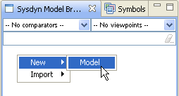
Rename the model to Population. Right-click on Model1 and select Rename.

Expand the model tree and double-click on Configuration. The model configuration diagram opens in a new editor.

Configuring the model structure

Our model is now empty. Let's build a population model for mice.

Open Symbols view and expand BasicSymbols. If BasicSymbols are not visible, make sure that you have the diagram open. The contents of the Symbols view depends on the active diagram editor.

Symbols view

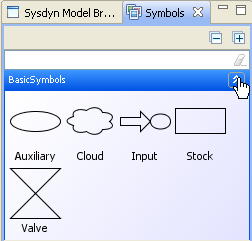
These are the basic symbols in System dynamics modelling. We will use these to create the model.

Drag one stock variable from Symbols view to the diagram. You can zoom and move on the diagram using shortcut keys.

Select the variable. Properties view on the bottom of the screen shows the properties of the selected variable. Change the name to Mice and press enter.

Stock variable Mice

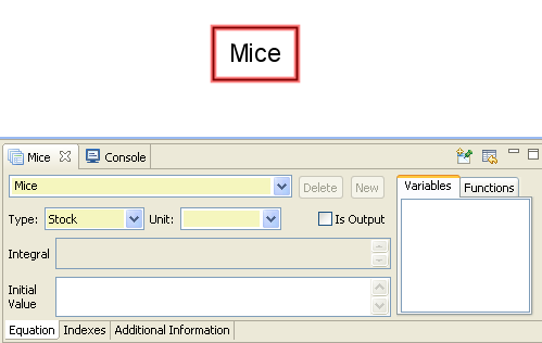
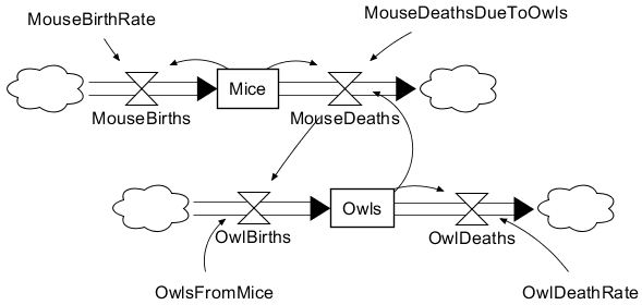
Next we will draw flows in and out of Mice. Hold down Alt and right-click on the left side of Mice. Move cursor on top of Mice and left-click. The system creates a Cloud where the flow starts, a flow from cloud to Mice and a valve in the middle of the flow. The valve controls the speed of the flow. Flow from Mice is created the same way. Hold down Alt. Right-click on Mice. Move cursor to the right of Mice and left-click. Rename the valves to MouseBirths and MouseDeaths.

Flows in and out of Mice

Of course mice are not alone in the world. There are also owls that hunt mice. Create a similar structure below mice for owls.

Owls and mice

To control the births and deaths, we need auxiliary variables. Auxiliary variables can be dragged from Symbols view just like Stock variables. We need one variable for each valve to control it. Drag the variables and rename them according to the picture below.

Auxiliaries for valves

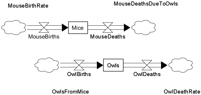
Arrow connections, dependencies, are created almost like flows. The difference is that the connection is started and ended with a left click and the connection can only be made between two existing variables. Connect the auxiliary variables and valves like in the picture below.

Dependency connections

Equations

As you can see from the model, we have made some shortcuts in our model to make it more simple. In reality, there are lots of other factors that affect mouse and owl populations. Let's however use this model as an example.

For the model to be simulated, each variable needs to have an equation. Equations can be configured from the property view, like the names. Input the following equations into the corresponding variables:

MouseBirths
= MouseBirthRate * Mice

MouseDeaths
= Mice * MouseDeathsDueToOwls * Owls

OwlBirths
= OwlsFromMice * MouseDeaths

OwlDeaths
= OwlDeathRate * Owls

MouseBirthRate
= 0.04

MouseDeathsDueToOwls
= 0.0005

OwlsFromMice
= 0.1

OwlDeathRate
= 0.09

Finally we need initial values for our populations.

Mice
Initial Value: 700

Owls
Initial Value: 10

Simulating the model

Experiment activation

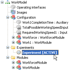
Now the model is configured and ready for simulation. Switch Symbols view back to Model Browser. Expand the Experiments folder on your model and double-click on Experiment. This activates the experiment. Experiment needs to be active before the model can be simulated. Experiment activations adds experiment control buttons to the toolbar. Press play to simulate the model.

System shows the simulation progress in the progress bar on the lower right corner of the screen.

When the progress indicator disappears, the simulation is complete.

After the simulation has run, you can select variables from the diagram or model browser and their values over the simulation time will be shown on Trend View. You can select multiple variables from the diagram by holding down Ctrl key. Select Mice and Owls.

Results for Mice and Owls

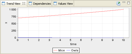
As you can see, the simulation is complete, but the results do not reveal any interesting behavior. Let's extend the simulation time.

Select Configuration from the model browser. In the properties-view change stop time to 300.0 and simulate again.

After the simualtion is complete, Select Mice and Owls again.

Results for Mice and Owls, Extended simulation time

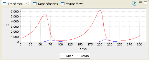
Now the simulation reveals the traditional behavior of predator-prey models. Feel free to adjust the parameters and try the simulations again.