Simantics System Dynamics

Simantics System Dynamics

Simantics System Dynamics is currently the only open source modelling and simulating tool for Simantics. Simantics System Dynamics is under development and will go through some changes in the future. New features will be added and old ones improved according to the needs of the modellers. New features include vector variables, module libraries and different analysis tools.

Some new features, like vector variables, may cause significant changes to the data structure of models in Simantics System Dynamics. Models created with current version may not be directly compatible with the future versions! However, if the future versions have significant changes, we try to create migration tools so that you can migrate our old models to the new versions.

This documentation introduces you to the current version of Simantics System Dynamics. Documentation includes the basic modelling principles and a guide on how to model system dynamics models with Simantics System Dynamics. If you like to get to know the tool better and try modelling and simulating yourself, install the software and try our basic and advanced tutorials!

Introduction to System Dynamics Simulation

System Dynamics

System dynamics is an approach to understanding different organizations, markets and other complex systems and their dynamic behavior. System dynamics modelling in Simantics is a free modelling tool. See installation instructions.

Model

Model structure

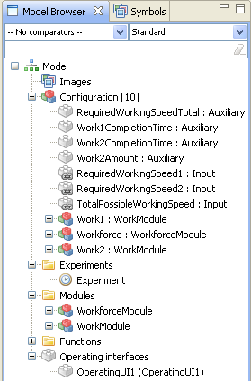
System dynamics model is generally understood as the model configuration. In this tool, the model contains also other components. Model can have Operating interfaces that enable the use of the model with simple controls. Operating interfaces are configured separately and when using them, the complex model is hidden from the user. Experiments are the way to simulate the model. In the future, you can have experiments with different configurations, for example different initial values for some parameters. In that way, you don't have to always configure the model for different scenarios. Modules folder contains all the different module types in your model and you can create new module types there.

Components

Most of the components you can use in your models are basic system dynamics components. The modularity of the models introduces two additional components, Modules and Inputs. All the components are explained below.

Component types

Auxiliary

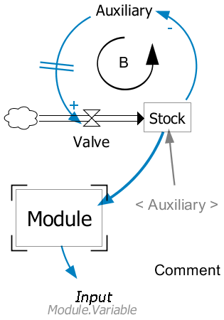
Auxiliary is the most basic variable you can use. It represents a single value or a mathematical expression. There are different types of auxiliary variables currently in the system: Auxiliary, Parameter, Constant and WithLookup. Auxiliary is the default type. Parameters are single values that the user can change. When only parameters are changed, the model simulates faster, because the system does not have to recompile the model. WithLookup is a special variable that has an expression and a lookup table. The expresssion defines what value is taken from the defined table.

Dependency

Dependency is an arrow that connects two components. It means that the value of the variable from which the arrow starts is used to calculate the value of the variable where the arrow ends.

Flow

Flow connects clouds, valves and stocks. Flow represents an actual flow of something from stocks or clouds to stocks or clouds. There has to be at least one valve in a flow and the system creates it automatically, if none of the ends of the flow is a valve.

Valve

Valve regulates the rate of a flow. The value of a valve is automatically used in calculating the level of an adjacent stock. Valves behave just like Auxiliary variables but look different and you can connect also flows to them.

Stock

The value of a stock variable is an integral of flows leaving and flows arriving to the variable. The integral is calculated automatically from the valves that are connected to the variable with flow connections. You must give an initial value to the stock. Initial value can be a single value or an equation. You can use values of other variables to calculate the initial value.

Cloud

Cloud is not a variable. It represents a starting or ending point of a flow, if it is not in the scope of the model.

Module

Modules enable structural modeling. Modules are defined just like the basic model configuration, but the module component hides the actual configuration. You can only connect dependency connections into the module and dependency connections from the module must end to Input variables. The interface of the module is defined using input and output variables in the configuration of the module. All variable types can be set as output variables. If a variable is an output variable, its font is bold.

Input

Input variables are the way of getting values from other modules. Inputs look like auxiliary variables except their font is italics. You can set a default value to the input variable in case it is not connected to any variable. Connections are made from the modules properties, when the module is populated. Input doesn't have to be connected with an arrow to a module. If the variable has no connections, it can get values from a higher level in the hierarchy. If an input is connected to an output, the output and its module are shown below the variable using dot notation.

Modeling principles

System dynamics modelling is much more than just mathematical formulas and nice graphs. Models are ways of communicating. There are some basic principles in system dynamics modelling that make the models easier to read and understand. You do not have to apply these principles to simulate models, but using them makes it easier for you to communicate your model to others.

Variable names

Variables names should be nouns, not verbs. The names should be positive: for example it is easier to understand that satisfaction decreases than dissatisfaction rises.

Variable names can and should have multiple words, if they are needed. Unfortunately current version of the tool does not support spaces in variable names. A good practice is to use CamelCase if name contains multiple words. This means that you start every word woth a capital letter (example: ExampleVariable).

Connections

You should try to avoid overlapping dependency arrows. In some situations, however, it is not possible. Dependencies should also form distinctive loops, if there is a loop. It makes it easier to read and understand the model and its behavior.

Graphical annotations

System dynamics contains usually annotations for loops, polarities, delays and so on. Currently those annotations are not supported, but the support will be added later. Annotations are important, again, for communicating the behavior of the model.

Installation Instructions

System dynamics tool is a provided with the Simantics platform.

1. Download installer from Simantics download page
2. Install the program to a directory without spaces.
3. Run Simantics-Sysdyn.exe
   

(Default path in windows: C:\Simantics\Sysdyn\1.2\simantics-sysdyn\Simantics-Sysdyn.exe)

OpenModelica is used to build and simulate the models. Simantics platform has integrated OpenModelica 1.5 for Windows environments. For other versions and other environments you need to install OpenModelica.

Workbench

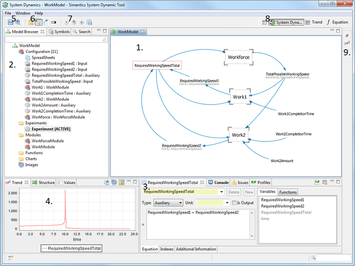
1. Diagram
   Diagram is the area where you will graphically modify your model. Diagrams are built from elements that can be dragged from Symbols view or populated using shortcut keys.
2. Model Browser
   Model browser shows the structure of your model and all items related to it.
   Symbols view is stacked with the model browser and used for dragging elements to diagrams.
3. Properties
   Property view shows the selected variable's properties. Property view has a different layout depending on the type of the selected component. The view can also have different tabs depending on the component type. Basic tabs are with variables are Equation and Additional information.
4. Trend
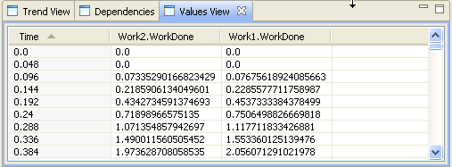
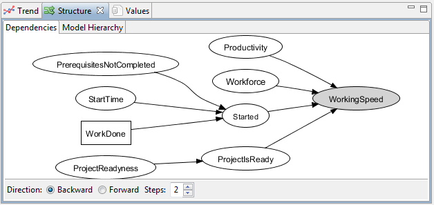
   Trend view shows the graphical representation of the values of the selected value over time. For the trend to be shown, a simulation has to be run. The view shows always the results of the latest run, but you can save results of a simulation and show them in the same trend with results from another simulation. Values view and Dependencies are stacked with Trend view and can also be used for analyzing the model.
5. Experiment controls
   Experiment controls are shown when an experiment is active. Experiment is activated by double clicking an experiment in the model browser. With the experiment control, you can start simulation runs and save simulation results.

Modelling

Basic modelling

Basic modelling functions enable you to create and configure models. System dynamics modeling is basically pretty simple, so with these instructions you can build small and also very large models. The tricky part is writing all the expressions and adjusting the model so that it actually tells you something.

Creating a new model

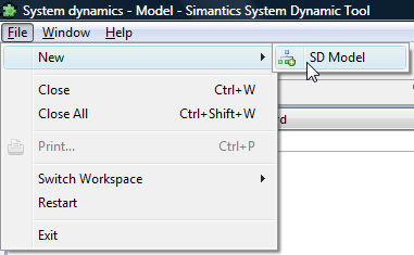
Start a new model by right-clicking the model browser and selecting New->Model or from the main menu File->New Model.

Creating a new module type

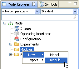
Create a new module type by right-clicking on the Modules-folder and selecting New->Module. This creates a new module type that you can populate to your other modules and the model configuration.

Configuring a model

Model configuration can be opened by double clicking Configuration in the model browser.

Configuring modules

Configuration of a module type can be opened by double clicking the module type you want to configure. You can also open the configuration of a module from a diagram, when a module has been populated to that diagram, by right-clicking the module and selecting Show Module. When opening modules from diagram, the opened diagram knows to which diagram the module has been populated and can show the connections between the modules. Keep in mind that when making changes to a module, the changes apply to all instances of the module!

Populate variables

You can drag variables to a diagram from symbol view. You can also populate variables using shortcut keys

Populate modules

Modules are populated from the model browser. Just drag the module you want to populate from the Modules folder to a diagram.

Create connections

There are two types of connections: dependencies and flows. Both are created basically the same way. Hold Alt down and click on a variable. Left click starts a dependency, right click starts a flow. Both are ended to another variable with a left click.

Flows can also be started and ended to an empty spot in the diagram. If there is no start or end variable, a cloud will be created. Also if start or end is not a valve, a new valve is created in the middle of the flow.

There are some restrictions on what connections can be made, but don't worry, the user interface won't let you do connections that are not allowed.

Connections between modules

Outside the module

You can connect variables to variables in modules like this:

MODULE -----> INPUT
or
ANY VARIABLE -----> MODULE 

This is just the visual configuration, but you need those connections to really connect variables in the module's properties.

In Inputs -tab you select which variables you connect to inputs inside the module. In Outputs -tab you select which variables you lift from the module to inputs outside it.

Inside the module

Input variables get values from outside the module

Output variables can send their values outside the module. From the variable properties, select Additional Information and press Is Output

Configure variables

Select a single variable from diagram or model browser. The properties of the variables are shown in the equation view and you can modify them.

Export model

To export your model to a file, select your model from the model browser, right-click and from the context menu choose Export... Select the folder where to export your model, give the file a name and press Save. You do not need to export a model to Save it, the model is automatically saved in your database. Export can be used to for example create different versions of the model, create backups or to transport it to another database.

Import model

Right-click on the model browser and select Import... Browse to your .tg file and select open. The model is added to your model browser.

Shortcut and control keys

Shortcut keys for configuring a model on diagram.

Shift + A	Hover Auxiliary at the cursor position, populate with left mouse button.
Shift + S	Hover Stock at the cursor position, populate with left mouse button.
Shift + C	Hover Cloud at the cursor position, populate with left mouse button.
Shift + V	Hover Valve at the cursor position, populate with left mouse button.
Shift + I	Hover Input at the cursor position, populate with left mouse button.
Alt + left mouse button	Start an arrow from a variable. End to another variable by clicking left mouse button.
Alt + right mouse button	Start flow from a variable. End by clicking left mouse button. If a flow is not started or ended on to a variable, a cloud will be created to that end. If a new flow does not have a valve at either end, a valve will be created in the middle of the flow.
Delete	Remove selected variables
Ctrl + left mouse button	Select multiple variables
Mouse wheel or + and -	Diagram zoom
drag(mouse3) or drag(shift + any mouse button)	Diagram pan
Ctrl + Z	Undo diagram action
Ctrl + Y	Redo diagram action
Ctrl + C	Copy selected elements
Ctrl + X	Cut selected elements
Ctrl + V	Paste copied or cut elements
G	Show / hide grid
R	Show / hide ruler

Other shortcut keys can be found selecting Window -> Preferences from the main menu. Keys are located in General -> Keys.

Simulation

Simulate model

To simulate a model, you need to activate an experiment. Browse to an experiment in you model browser and double click on the experiment. Experiment controls appear to the main tool bar. Click on the play button to run a simulation.

Analyze results

There are currently three analysis tools in the system dynamics tool.

Trend

Shows you the values of the selected variable(s) graphically over the simulation time. You can modify the trend and zoom it using the context menu (right-click) of the trend.

Values

Shows you the values of the selected variable(s) in a table form. If the value has a star (*) at the end, it means that the value is an approximate. There is no value for that variable for the given time step.

Dependencies

Dependencies is not actually an analysis tool for simulation results. It can show even without simulation which variables affect and which are affected by the selected variable. The direction and number of steps that are traveled from the selected variable can be selected at the bottom of the view.

Compare results

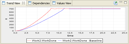
You can compare different results of the same model by saving simulation results and displaying the saved results side by side with other results. You can save your results after simulating by clicking the save button on your experiment controls. The saved results appear to model browser under the active experiment. To show the results on trends and tables, right-click on the result and select Show on charts.

Operating Interfaces

How interfaces can be created, how they can be used, current components

Create

Right-click on Operating interfaces and select New->Operating UI. Open the Operating User Interface by double clicking it.

Configure

Operating UIs have their own set of widgets. Widget symbols can be seen in the Symbols view and dragged to the diagram. The properties of the widgets can be modified from the properties view (same as equation view).

To connect a variable to a widget, just drag it from the model browser to the widget.

You can use monitors as labels, but to change the text on the monitor, you have to switch to operating mode by clicking .

Use

To use the interface you have created, you have to switch to operating mode by clicking . Activate a simulation, run it and the trends will show the results. You can switch values of parameters with the widgets and simulate again.

Multidimensional variables

Modeling

Models with multidimensional variables look just like any other models. The structure of the models is replicated givin multiple indexes to variables. For users with programming background, notation Variable[] may be familiar. In system dynamic modeling we need to give names to the indexes. Instead of using numbers to define the indexes, like in normal programming, we use enumerations. The steps to create a model with multidimensional variables are as follows (with examples):

1. Create the model structure
   Model with multidimensional variables looks just like any other model.
   
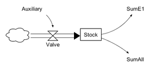
2. Create Enumerations and define the indexes
   Enumerations are created by right-clicking configuration and selecting New->Enumeration.
   
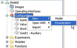
   Define enumeration indexes by adding as many indexes as you want. Rename the indexes by selecting them and then clicking on them again.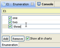
   
3. Add Enumerations for variables
   Select the variable that you want to be multidimensional. From the Indexes -tab in the property view, move the wanted enumerations to the right. The order of the enumerations does matter.
4. Define equations for all possible indexes
   Multidimensional variable can be thought as a multidimensional table. Each cell of the table needs to have an expression or a value. A cell cannot have multiple definitions. All cells can be defined in one expression like in the following example. E1 and E2 have both three indexes, so the resulting definition can be {{1,2,3},{4,5,6},{7,8,9}}.
   

Expressions

Values for all cells in the variable matrix can be defined in a single expression.

In many situations, it is however more clear to define separate expressions for each cell or blocks.

1. Define range for the expression
   
2. Define the expression (dimensions of the defined range and the result of the expression must match!)
   
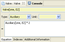
3. Create a new expression
   
4. Select the new expression
   

Loop this until there is value for each cell. There must be exactly one value for each cell.

Arithmetic Operators

Elementwise and Matrix operators

Builtin functions

ndims(A) size(A, i) size(A)

zeros(n1,n2,n3) ones(n1,n2,n3) fill(s,n1,n2,n3)

min(A) max(A) sum(A) product(A)

Simantics | System Dynamics Modelling

---

Tutorial: Basic System Dynamics Modelling
System dynamics modelling in Simantics is a free modelling tool that is included into the basic installation. This tutorial introduces the basic features of the system dynamics modelling tool.

Tutorial: Advanced System Dynamics Modelling
This tutorial introduces the more advanced features of the system dynamics modelling tool: Modules and Operating interfaces